Segment Tree

Overview

A Segment Tree is a data structure that stores information about array intervals as a tree. This allows answering range queries over an array efficiently, while still being flexible enough to allow quick modification of the array. This includes finding the sum of consecutive array elements $a[l \dots r]$ , or finding the minimum element in a such a range in $O(\log n)$ time. Between answering such queries, the Segment Tree allows modifying the array by replacing one element, or even changing the elements of a whole subsegment (e.g. assigning all elements $a[l \dots r]$ to any value, or adding a value to all element in the subsegment).

In general, a Segment Tree is a very flexible data structure, and a huge number of problems can be solved with it. Additionally, it is also possible to apply more complex operations and answer more complex queries (see Advanced versions of Segment Trees). In particular the Segment Tree can be easily generalized to larger dimensions. For instance, with a two-dimensional Segment Tree you can answer sum or minimum queries over some subrectangle of a given matrix in only $O(\log^2 n)$ time.

One important property of Segment Trees is that they require only a linear amount of memory. The standard Segment Tree requires $4n$ vertices for working on an array of size $n$ .

Simplest form of a Segment Tree

To start easy, we consider the simplest form of a Segment Tree. We want to answer sum queries efficiently. The formal definition of our task is: Given an array $a[0 \dots n-1]$ , the Segment Tree must be able to find the sum of elements between the indices $l$ and $r$ (i.e. computing the sum $\sum_{i=l}^r a[i]$ ), and also handle changing values of the elements in the array (i.e. perform assignments of the form $a[i] = x$ ). The Segment Tree should be able to process both queries in $O(\log n)$ time.

This is an improvement over the simpler approaches. A naive array implementation - just using a simple array - can update elements in $O(1)$ , but requires $O(n)$ to compute each sum query. And precomputed prefix sums can compute sum queries in $O(1)$ , but updating an array element requires $O(n)$ changes to the prefix sums.

Structure of the Segment Tree

We can take a divide-and-conquer approach when it comes to array segments. We compute and store the sum of the elements of the whole array, i.e. the sum of the segment $a[0 \dots n-1]$ . We then split the array into two halves $a[0 \dots n/2-1]$ and $a[n/2 \dots n-1]$ and compute the sum of each halve and store them. Each of these two halves in turn are split in half, and so on until all segments reach size $1$ .

We can view these segments as forming a binary tree: the root of this tree is the segment $a[0 \dots n-1]$ , and each vertex (except leaf vertices) has exactly two child vertices. This is why the data structure is called “Segment Tree”, even though in most implementations the tree is not constructed explicitly (see Implementation).

Here is a visual representation of such a Segment Tree over the array $a = [1, 3, -2, 8, -7]$ :

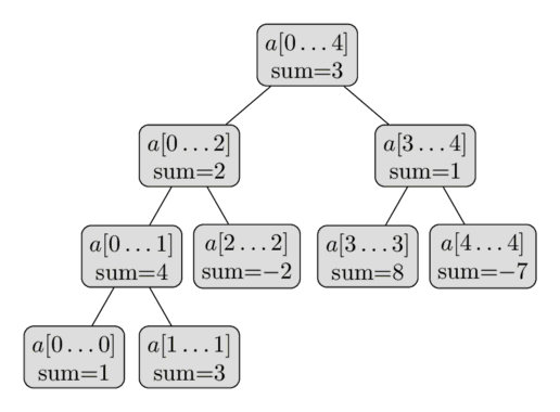
From this short description of the data structure, we can already conclude that a Segment Tree only requires a linear number of vertices. The first level of the tree contains a single node (the root), the second level will contain two vertices, in the third it will contain four vertices, until the number of vertices reaches $n$ . Thus the number of vertices in the worst case can be estimated by the sum $1 + 2 + 4 + \dots + 2^{\lceil\log_2 n\rceil} \lt 2^{\lceil\log_2 n\rceil + 1} \lt 4n$ .

It is worth noting that whenever $n$ is not a power of two, not all levels of the Segment Tree will be completely filled. We can see that behavior in the image. For now we can forget about this fact, but it will become important later during the implementation.

The height of the Segment Tree is $O(\log n)$ , because when going down from the root to the leaves the size of the segments decreases approximately by half.

Construction

Before constructing the segment tree, we need to decide:

the value that gets stored at each node of the segment tree. For example, in a sum segment tree, a node would store the sum of the elements in its range $[l, r]$ .
the merge operation that merges two siblings in a segment tree. For example, in a sum segment tree, the two nodes corresponding to the ranges $a[l_1 \dots r_1]$ and $a[l_2 \dots r_2]$ would be merged into a node corresponding to the range $a[l_1 \dots r_2]$ by adding the values of the two nodes.

Note that a vertex is a “leaf vertex”, if its corresponding segment covers only one value in the original array. It is present at the lowermost level of a segment tree. Its value would be equal to the (corresponding) element $a[i]$ .

Now, for construction of the segment tree, we start at the bottom level (the leaf vertices) and assign them their respective values. On the basis of these values, we can compute the values of the previous level, using the merge function. And on the basis of those, we can compute the values of the previous, and repeat the procedure until we reach the root vertex.

It is convenient to describe this operation recursively in the other direction, i.e., from the root vertex to the leaf vertices. The construction procedure, if called on a non-leaf vertex, does the following:

recursively construct the values of the two child vertices
merge the computed values of these children.

We start the construction at the root vertex, and hence, we are able to compute the entire segment tree.

The time complexity of this construction is $O(n)$ , assuming that the merge operation is constant time (the merge operation gets called $n$ times, which is equal to the number of internal nodes in the segment tree).

Sum queries

For now we are going to answer sum queries. As an input we receive two integers $l$ and $r$ , and we have to compute the sum of the segment $a[l \dots r]$ in $O(\log n)$ time.

To do this, we will traverse the Segment Tree and use the precomputed sums of the segments. Let’s assume that we are currently at the vertex that covers the segment $a[tl \dots tr]$ . There are three possible cases.

The easiest case is when the segment $a[l \dots r]$ is equal to the corresponding segment of the current vertex (i.e. $a[l \dots r] = a[tl \dots tr]$ ), then we are finished and can return the precomputed sum that is stored in the vertex.

Alternatively the segment of the query can fall completely into the domain of either the left or the right child. Recall that the left child covers the segment $a[tl \dots tm]$ and the right vertex covers the segment $a[tm + 1 \dots tr]$ with $tm = (tl + tr) / 2$ . In this case we can simply go to the child vertex, which corresponding segment covers the query segment, and execute the algorithm described here with that vertex.

And then there is the last case, the query segment intersects with both children. In this case we have no other option as to make two recursive calls, one for each child. First we go to the left child, compute a partial answer for this vertex (i.e. the sum of values of the intersection between the segment of the query and the segment of the left child), then go to the right child, compute the partial answer using that vertex, and then combine the answers by adding them. In other words, since the left child represents the segment $a[tl \dots tm]$ and the right child the segment $a[tm+1 \dots tr]$ , we compute the sum query $a[l \dots tm]$ using the left child, and the sum query $a[tm+1 \dots r]$ using the right child.

So processing a sum query is a function that recursively calls itself once with either the left or the right child (without changing the query boundaries), or twice, once for the left and once for the right child (by splitting the query into two subqueries). And the recursion ends, whenever the boundaries of the current query segment coincides with the boundaries of the segment of the current vertex. In that case the answer will be the precomputed value of the sum of this segment, which is stored in the tree.

In other words, the calculation of the query is a traversal of the tree, which spreads through all necessary branches of the tree, and uses the precomputed sum values of the segments in the tree.

Obviously we will start the traversal from the root vertex of the Segment Tree.

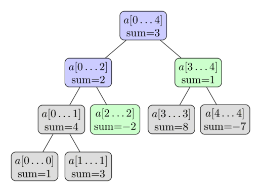
The procedure is illustrated in the following image. Again the array $a = [1, 3, -2, 8, -7]$ is used, and here we want to compute the sum $\sum_{i=2}^4 a[i]$ . The colored vertices will be visited, and we will use the precomputed values of the green vertices. This gives us the result $-2 + 1 = -1$ .

Why is the complexity of this algorithm $O(\log n)$ ? To show this complexity we look at each level of the tree. It turns out, that for each level we only visit not more than four vertices. And since the height of the tree is $O(\log n)$ , we receive the desired running time.

We can show that this proposition (at most four vertices each level) is true by induction. At the first level, we only visit one vertex, the root vertex, so here we visit less than four vertices. Now let’s look at an arbitrary level. By induction hypothesis, we visit at most four vertices. If we only visit at most two vertices, the next level has at most four vertices. That trivial, because each vertex can only cause at most two recursive calls. So let’s assume that we visit three or four vertices in the current level. From those vertices, we will analyze the vertices in the middle more carefully. Since the sum query asks for the sum of a continuous subarray, we know that segments corresponding to the visited vertices in the middle will be completely covered by the segment of the sum query. Therefore these vertices will not make any recursive calls. So only the most left, and the most right vertex will have the potential to make recursive calls. And those will only create at most four recursive calls, so also the next level will satisfy the assertion. We can say that one branch approaches the left boundary of the query, and the second branch approaches the right one.

Therefore we visit at most $4 \log n$ vertices in total, and that is equal to a running time of $O(\log n)$ .

In conclusion the query works by dividing the input segment into several sub-segments for which all the sums are already precomputed and stored in the tree. And if we stop partitioning whenever the query segment coincides with the vertex segment, then we only need $O(\log n)$ such segments, which gives the effectiveness of the Segment Tree.

Update queries

Now we want to modify a specific element in the array, let’s say we want to do the assignment $a[i] = x$ . And we have to rebuild the Segment Tree, such that it correspond to the new, modified array.

This query is easier than the sum query. Each level of a Segment Tree forms a partition of the array. Therefore an element $a[i]$ only contributes to one segment from each level. Thus only $O(\log n)$ vertices need to be updated.

It is easy to see, that the update request can be implemented using a recursive function. The function gets passed the current tree vertex, and it recursively calls itself with one of the two child vertices (the one that contains $a[i]$ in its segment), and after that recomputes its sum value, similar how it is done in the build method (that is as the sum of its two children).

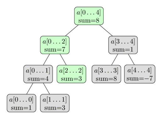
Again here is a visualization using the same array. Here we perform the update $a[2] = 3$ . The green vertices are the vertices that we visit and update.

Implementation

The main consideration is how to store the Segment Tree. Of course we can define a $\text{Vertex}$ struct and create objects, that store the boundaries of the segment, its sum and additionally also pointers to its child vertices. However, this requires storing a lot of redundant information in the form of pointers. We will use a simple trick to make this a lot more efficient by using an implicit data structure: Only storing the sums in an array. (A similar method is used for binary heaps). The sum of the root vertex at index 1, the sums of its two child vertices at indices 2 and 3, the sums of the children of those two vertices at indices 4 to 7, and so on. With 1-indexing, conveniently the left child of a vertex at index $i$ is stored at index $2i$ , and the right one at index $2i + 1$ . Equivalently, the parent of a vertex at index $i$ is stored at $i/2$ (integer division).

This simplifies the implementation a lot. We don’t need to store the structure of the tree in memory. It is defined implicitly. We only need one array which contains the sums of all segments.

As noted before, we need to store at most $4n$ vertices. It might be less, but for convenience we always allocate an array of size $4n$ . There will be some elements in the sum array, that will not correspond to any vertices in the actual tree, but this doesn’t complicate the implementation.

So, we store the Segment Tree simply as an array $t[]$ with a size of four times the input size $n$ :

1

int n, t[4*MAXN];

The procedure for constructing the Segment Tree from a given array $a[\ ]$ looks like this: it is a recursive function with the parameters $a[\ ]$ (the input array), $v$ (the index of the current vertex), and the boundaries $tl$ and $tr$ of the current segment. In the main program this function will be called with the parameters of the root vertex: $v = 1$ , $tl = 0$ , and $tr = n - 1$ .

 1
 2
 3
 4
 5
 6
 7
 8
 9
10


void build(int a[], int v, int tl, int tr) {
    if (tl == tr) {
        t[v] = a[tl];
    } else {
        int tm = (tl + tr) / 2;
        build(a, v*2, tl, tm);
        build(a, v*2+1, tm+1, tr);
        t[v] = t[v*2] + t[v*2+1];
    }
}

Further the function for answering sum queries is also a recursive function, which receives as parameters information about the current vertex/segment (i.e. the index $v$ and the boundaries $tl$ and $tr$ ) and also the information about the boundaries of the query, $l$ and $r$ . In order to simplify the code, this function always does two recursive calls, even if only one is necessary - in that case the superfluous recursive call will have $l > r$ , and this can easily be caught using an additional check at the beginning of the function.

 1
 2
 3
 4
 5
 6
 7
 8
 9
10


int sum(int v, int tl, int tr, int l, int r) {
    if (l > r)
        return 0;
    if (l == tl && r == tr) {
        return t[v];
    }
    int tm = (tl + tr) / 2;
    return sum(v*2, tl, tm, l, min(r, tm))
           + sum(v*2+1, tm+1, tr, max(l, tm+1), r);
}

Finally the update query. The function will also receive information about the current vertex/segment, and additionally also the parameter of the update query (i.e. the position of the element and its new value).

 1
 2
 3
 4
 5
 6
 7
 8
 9
10
11
12


void update(int v, int tl, int tr, int pos, int new_val) {
    if (tl == tr) {
        t[v] = new_val;
    } else {
        int tm = (tl + tr) / 2;
        if (pos <= tm)
            update(v*2, tl, tm, pos, new_val);
        else
            update(v*2+1, tm+1, tr, pos, new_val);
        t[v] = t[v*2] + t[v*2+1];
    }
}

Memory efficient implementation

Most people use the implementation from the previous section. If you look at the array t you can see that it follows the numbering of the tree nodes in the order of a BFS traversal (level-order traversal). Using this traversal the children of vertex $v$ are $2v$ and $2v + 1$ respectively. However if $n$ is not a power of two, this method will skip some indices and leave some parts of the array t unused. The memory consumption is limited by $4n$ , even though a Segment Tree of an array of $n$ elements requires only $2n - 1$ vertices.

However it can be reduced. We renumber the vertices of the tree in the order of an Euler tour traversal (pre-order traversal), and we write all these vertices next to each other.

Lets look at a vertex at index $v$ , and let him be responsible for the segment $[l, r]$ , and let $mid = \dfrac{l + r}{2}$ . It is obvious that the left child will have the index $v + 1$ . The left child is responsible for the segment $[l, mid]$ , i.e. in total there will be $2 * (mid - l + 1) - 1$ vertices in the left child’s subtree. Thus we can compute the index of the right child of $v$ . The index will be $v + 2 * (mid - l + 1)$ . By this numbering we achieve a reduction of the necessary memory to $2n$ .

Advanced versions of Segment Trees

A Segment Tree is a very flexible data structure, and allows variations and extensions in many different directions. Let’s try to categorize them below.

More complex queries

It can be quite easy to change the Segment Tree in a direction, such that it computes different queries (e.g. computing the minimum / maximum instead of the sum), but it also can be very nontrivial.

Finding the maximum

Let us slightly change the condition of the problem described above: instead of querying the sum, we will now make maximum queries.

The tree will have exactly the same structure as the tree described above. We only need to change the way $t[v]$ is computed in the $\text{build}$ and $\text{update}$ functions. $t[v]$ will now store the maximum of the corresponding segment. And we also need to change the calculation of the returned value of the $\text{sum}$ function (replacing the summation by the maximum).

Of course this problem can be easily changed into computing the minimum instead of the maximum.

Instead of showing an implementation to this problem, the implementation will be given to a more complex version of this problem in the next section.

Finding the maximum and the number of times it appears

This task is very similar to the previous one. In addition of finding the maximum, we also have to find the number of occurrences of the maximum.

To solve this problem, we store a pair of numbers at each vertex in the tree: In addition to the maximum we also store the number of occurrences of it in the corresponding segment. Determining the correct pair to store at $t[v]$ can still be done in constant time using the information of the pairs stored at the child vertices. Combining two such pairs should be done in a separate function, since this will be an operation that we will do while building the tree, while answering maximum queries and while performing modifications.

 1
 2
 3
 4
 5
 6
 7
 8
 9
10
11
12
13
14
15
16
17
18
19
20
21
22
23
24
25
26
27
28
29
30
31
32
33
34
35
36
37
38
39
40
41
42
43


pair<int, int> t[4*MAXN];

pair<int, int> combine(pair<int, int> a, pair<int, int> b) {
    if (a.first > b.first)
        return a;
    if (b.first > a.first)
        return b;
    return make_pair(a.first, a.second + b.second);
}

void build(int a[], int v, int tl, int tr) {
    if (tl == tr) {
        t[v] = make_pair(a[tl], 1);
    } else {
        int tm = (tl + tr) / 2;
        build(a, v*2, tl, tm);
        build(a, v*2+1, tm+1, tr);
        t[v] = combine(t[v*2], t[v*2+1]);
    }
}

pair<int, int> get_max(int v, int tl, int tr, int l, int r) {
    if (l > r)
        return make_pair(-INF, 0);
    if (l == tl && r == tr)
        return t[v];
    int tm = (tl + tr) / 2;
    return combine(get_max(v*2, tl, tm, l, min(r, tm)),
                   get_max(v*2+1, tm+1, tr, max(l, tm+1), r));
}

void update(int v, int tl, int tr, int pos, int new_val) {
    if (tl == tr) {
        t[v] = make_pair(new_val, 1);
    } else {
        int tm = (tl + tr) / 2;
        if (pos <= tm)
            update(v*2, tl, tm, pos, new_val);
        else
            update(v*2+1, tm+1, tr, pos, new_val);
        t[v] = combine(t[v*2], t[v*2+1]);
    }
}

Compute the greatest common divisor / least common multiple

In this problem we want to compute the GCD / LCM of all numbers of given ranges of the array.

This interesting variation of the Segment Tree can be solved in exactly the same way as the Segment Trees we derived for sum / minimum / maximum queries: it is enough to store the GCD / LCM of the corresponding vertex in each vertex of the tree. Combining two vertices can be done by computing the GCD / LCM of both vertices.

Counting the number of zeros, searching for the k-th zero

In this problem we want to find the number of zeros in a given range, and additionally find the index of the $k$ -th zero using a second function.

Again we have to change the store values of the tree a bit: This time we will store the number of zeros in each segment in $t[]$ . It is pretty clear, how to implement the $\text{build}$ , $\text{update}$ and $\text{count\_zero}$ functions, we can simply use the ideas from the sum query problem. Thus we solved the first part of the problem.

Now we learn how to solve the problem of finding the $k$ -th zero in the array $a[]$ . To do this task, we will descend the Segment Tree, starting at the root vertex, and moving each time to either the left or the right child, depending on which segment contains the $k$ -th zero. In order to decide to which child we need to go, it is enough to look at the number of zeros appearing in the segment corresponding to the left vertex. If this precomputed count is greater or equal to $k$ , it is necessary to descend to the left child, and otherwise descent to the right child. Notice, if we chose the right child, we have to subtract the number of zeros of the left child from $k$ .

In the implementation we can handle the special case, $a[]$ containing less than $k$ zeros, by returning -1.